What is Linear Regression
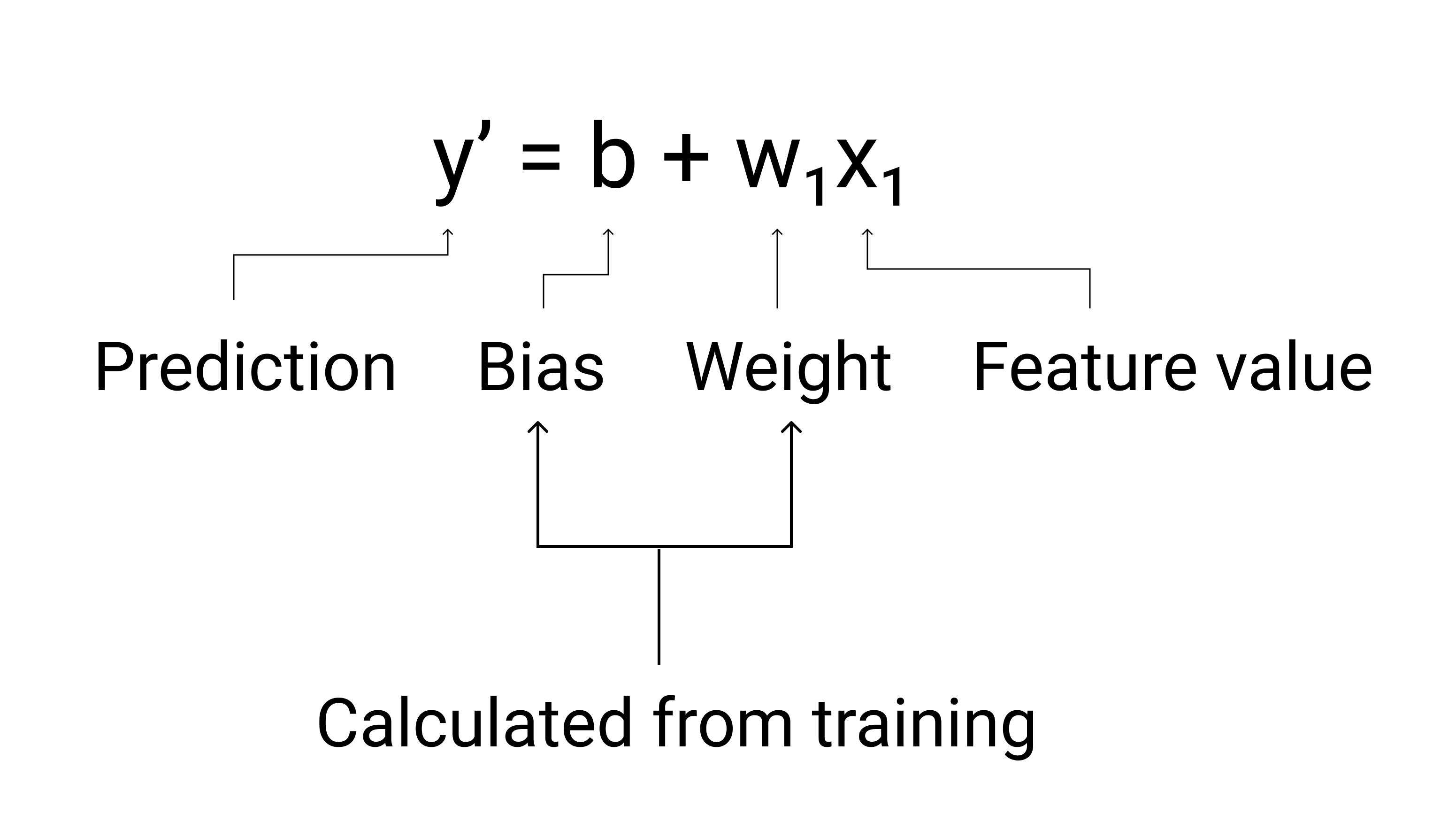
Training data to form a model, simply say, it is to find the bias and weights among the data. linear regression is one of the methods that find the relationship between features and a label to get the bias and weights.
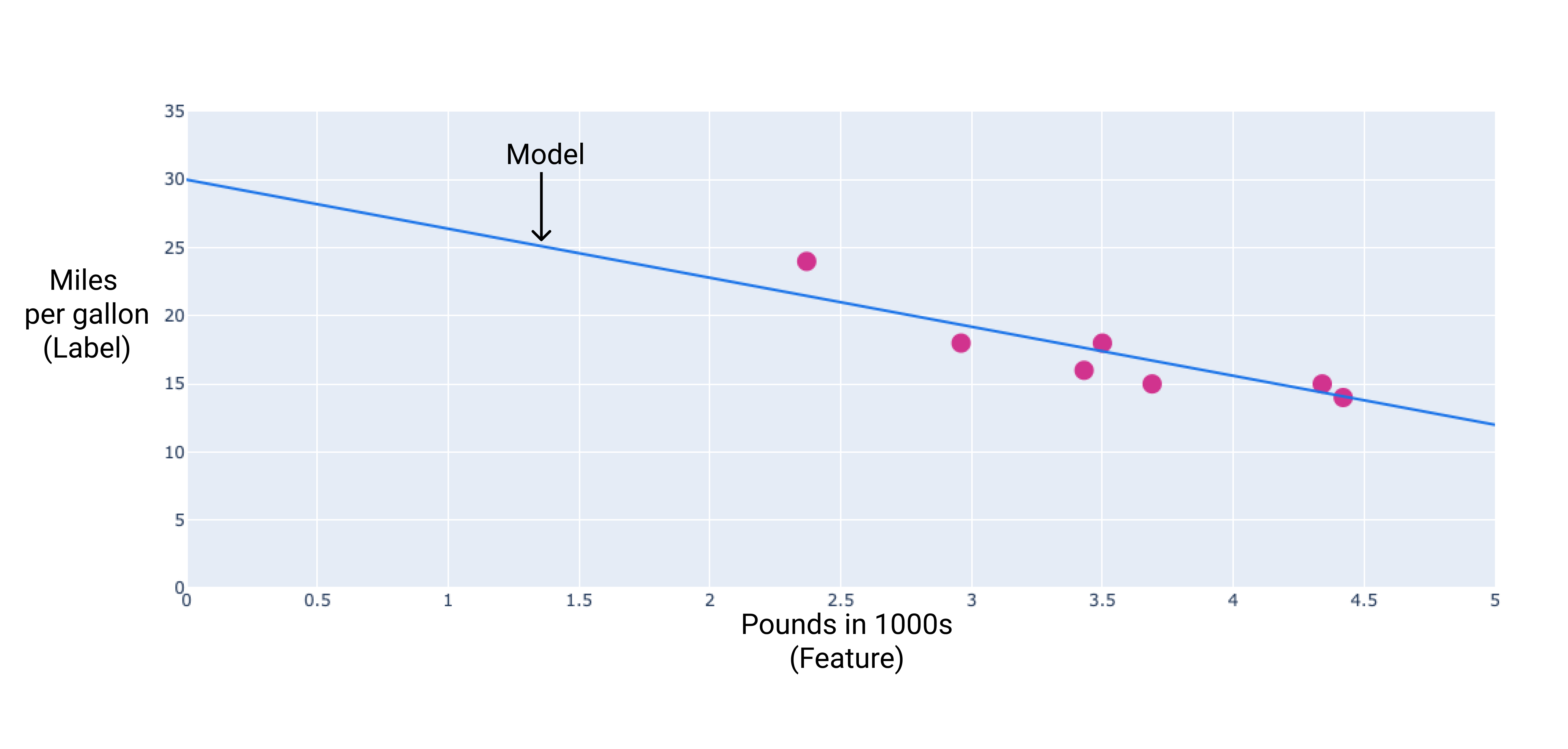
During training, the model calculates the weight and bias that produce the best model.
Loss
Loss is a numerical metric that describes how wrong a model’s predictions are. Loss measures the distance between the model’s predictions and the actual labels. The goal of training a model is to minimize the loss, reducing it to its lowest possible value.
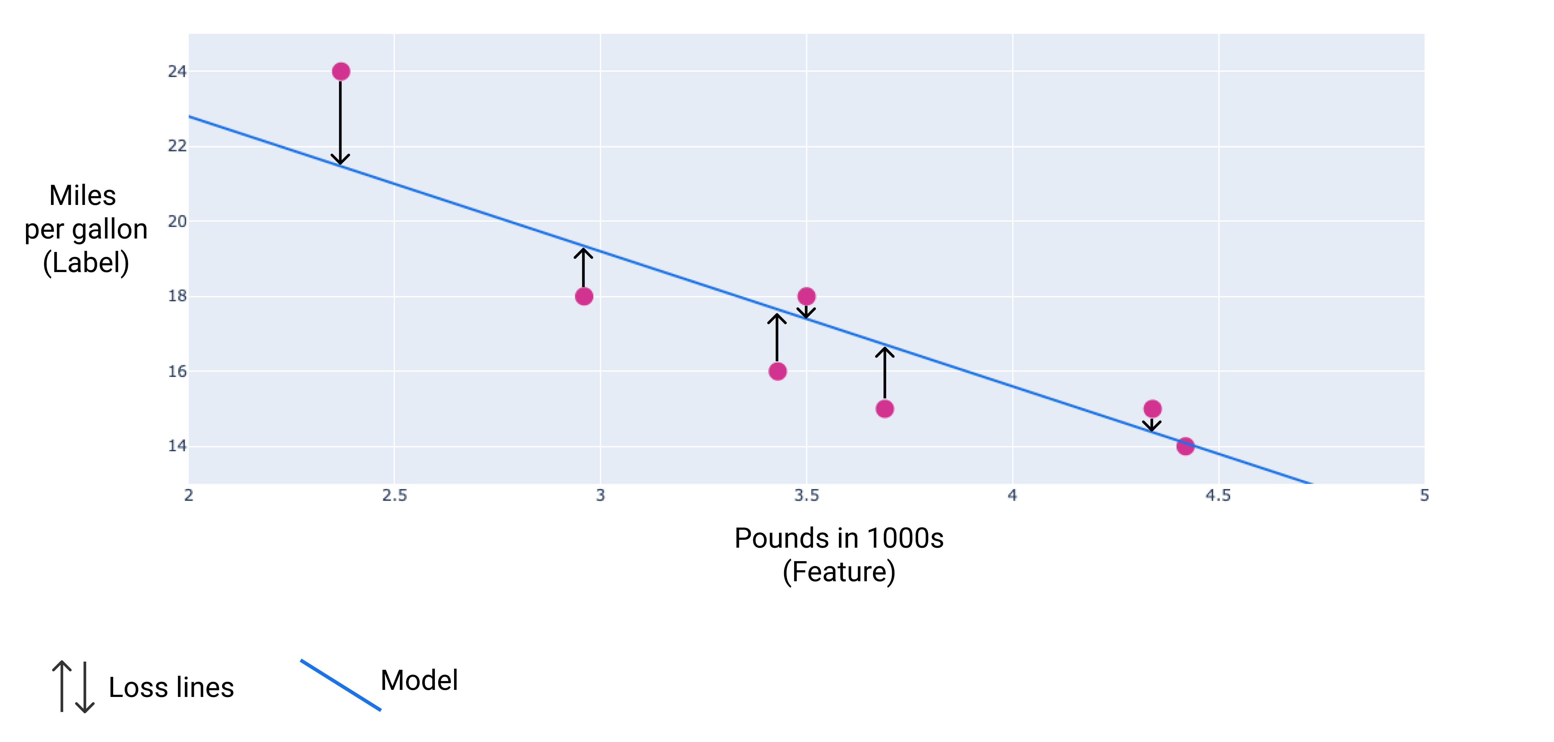
The two most common methods to remove the sign are the following:
- Take the absolute value of the difference between the actual value and the prediction.
- Square the difference between the actual value and the prediction.
There are four main types of loss:
- L1 loss: The sum of the absolute values of the difference between the predicted values and the actual values.
- Mean absolute error (MAE): The average of L1 losses across a set of examples.
- L2 loss: The sum of the squared difference between the predicted values and the actual values.
- Mean squared error (MSE): The average of L2 losses across a set of examples.
Choosing a loss
In training, model will try to get the best bias and weights according to the LOSS. So choosing a loss is matter.
When choosing the best loss function, also consider how you want the model to treat outliers. The outliers are closer to the model trained with MSE than to the model trained with MAE.
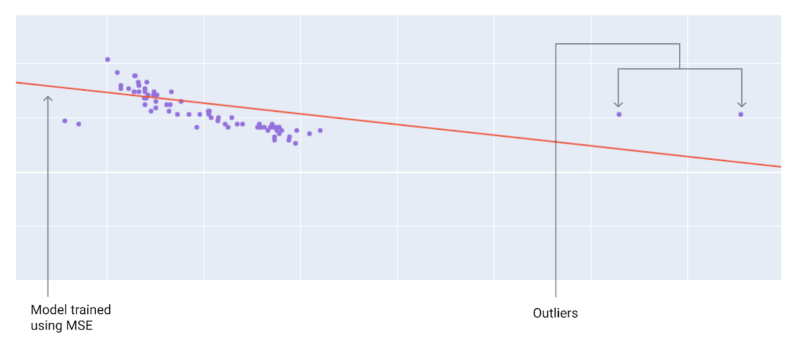
A model trained with MSE moves the model closer to the outliers.
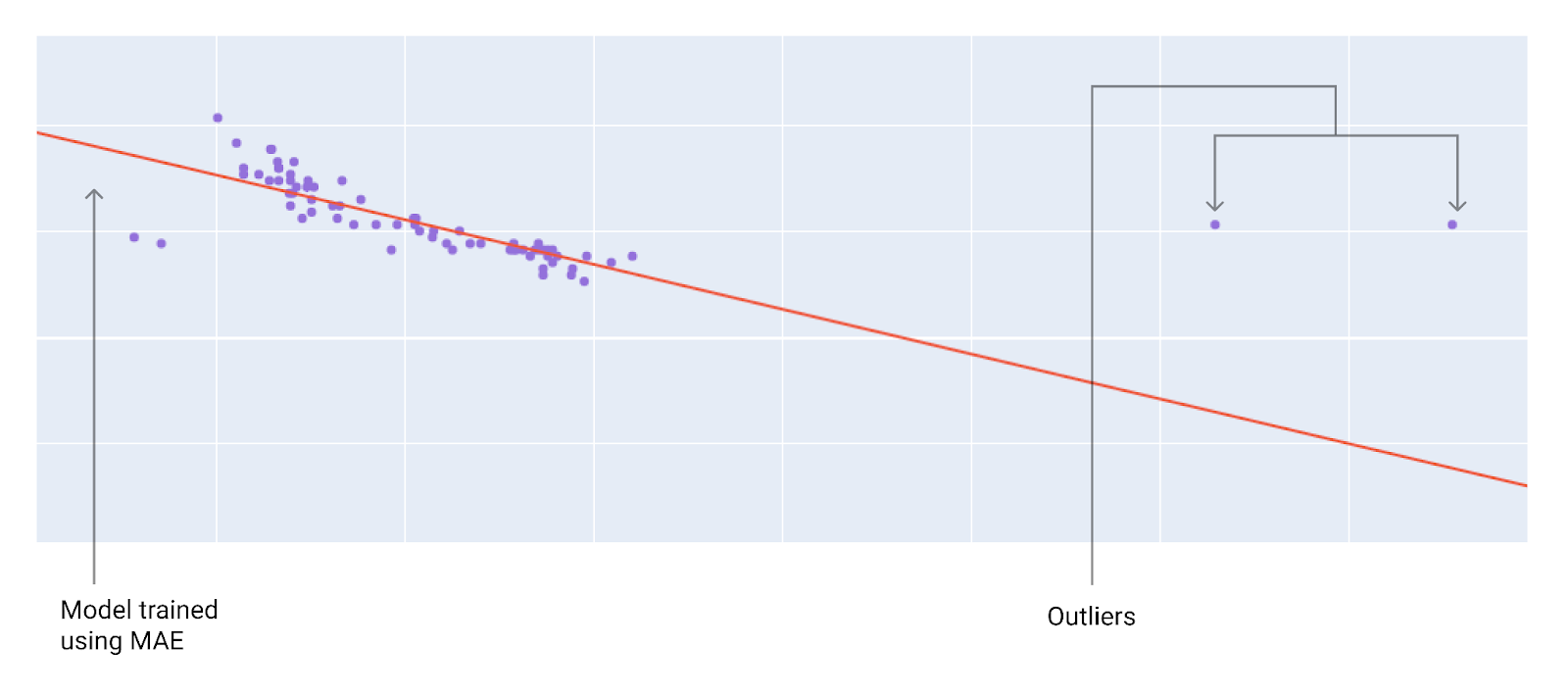
A model trained with MAE is farther from the outliers.
Gradient descent
Gradient descent is a mathematical technique that iteratively finds the weights and bias that produce the model with the lowest loss.
Gradient descent finds the best weight and bias by repeating the following process for a number of user-defined iterations. The model begins training with randomized weights and biases near zero, and then repeats the following steps:
- Calculate the loss with the current weight and bias.
- Determine the direction to move the weights and bias that reduce loss.
- Move the weight and bias values a small amount in the direction that reduces loss.
- Return to step one and repeat the process until the model can’t reduce the loss any further.
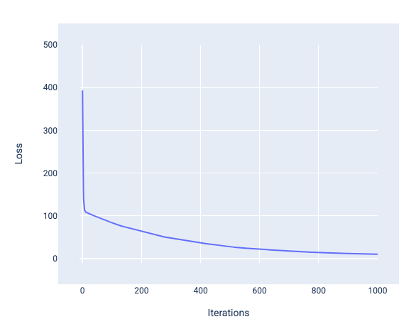
This is typical loss curve, Loss is on the y-axis and iterations are on the x-axis:
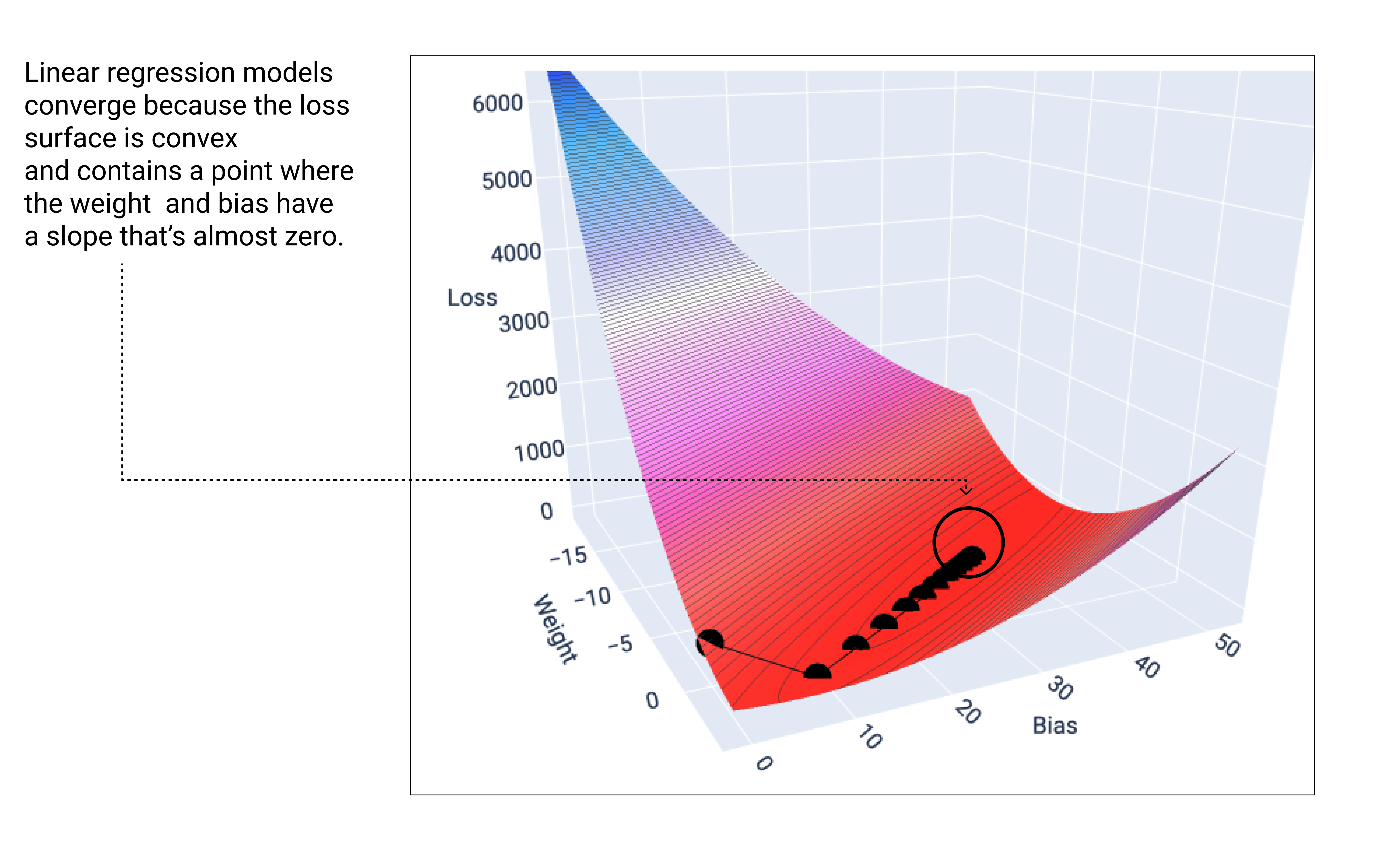
Loss surface showing the weight and bias values that produce the lowest loss.
Hyperparameters
Hyperparameters are variables that control different aspects of training. Three common hyperparameters are:
- Learning rate
- Batch size
- Epochs
In contrast, parameters are the variables, like the weights and bias, that are part of the model itself. In other words, hyperparameters are values that you control; parameters are values that the model calculates during training.
Learning rate
The learning rate determines the magnitude of the changes to make to the weights and bias during each step of the gradient descent process.
The model multiplies the gradient by the learning rate to determine the model’s parameters (weight and bias values) for the next iteration. For example, if the gradient’s magnitude is 2.5 and the learning rate is 0.01, then the model will change the parameter by 0.025.
Learning rate is a floating point number you set that influences how quickly the model converges.
The ideal learning rate helps the model to converge within a reasonable number of iterations.
What do it means when Learning Rate is 1?
A learning rate of 1 means that the model updates its weights by the full amount of the calculated gradient. This almost inevitably leads to highly unstable training and the model failing to converge to a good solution.
Batch size
Batch size is a hyperparameter that refers to the number of examples the model processes before updating its weights and bias.
You might think that the model should do Full Batch, means calculating the loss for every example in the dataset before updating the weights and bias. However, when a dataset contains hundreds of thousands or even millions of examples, using the full batch isn’t practical.
Two common techniques to get the right gradient on average without needing to look at every example in the dataset before updating the weights and bias:
- Stochastic gradient descent (SGD): Stochastic gradient descent uses only a single example (a batch size of one) per iteration. The term “stochastic” indicates that the one example comprising each batch is chosen at random. (Note that using stochastic gradient descent can produce noise throughout the entire loss curve, not just near convergence.)
- Mini-batch stochastic gradient descent (mini-batch SGD): Mini-batch stochastic gradient descent is a compromise between full-batch and SGD. The model chooses the examples included in each batch at random, averages their gradients, and then updates the weights and bias once per iteration.
Epochs
During training, an epoch means that the model has processed every example in the training set once. For example, given a training set with 1,000 examples and a mini-batch size of 100 examples, it will take the model 10 iterations to complete one epoch.
Training typically requires many epochs. In general, more epochs produces a better model, but also takes more time to train.
Here is an example to tell the difference:
- Full batch: After the model looks at all the examples in the dataset. For instance, if a dataset contains 1,000 examples and the model trains for 20 epochs, the model updates the weights and bias 20 times, once per epoch.
- Stochastic gradient descent: After the model looks at a single example from the dataset. For instance, if a dataset contains 1,000 examples and trains for 20 epochs, the model updates the weights and bias 20,000 times.
- Mini-batch stochastic gradient descent: After the model looks at the examples in each batch. For instance, if a dataset contains 1,000 examples, and the batch size is 100, and the model trains for 20 epochs, the model updates the weights and bias 200 times.
Generate a correlation matrix
An important part of machine learning is determining which features correlate with the label. you can use a correlation matrix to identify features whose values correlate well with the label.
Correlation values have the following meanings:
- 1.0: perfect positive correlation; that is, when one attribute rises, the other attribute rises.
- -1.0: perfect negative correlation; that is, when one attribute rises, the other attribute falls.
- 0.0: no correlation; the two columns are not linearly related.
In general, the higher the absolute value of a correlation value, the greater its predictive power.
Pandas’s dataframe provide such function:
training_df.corr(numeric_only = True)
Visualize relationships in dataset
Pandas’s dataframe provide function to visualize:
sns.pairplot(training_df, x_vars=["FARE", "TRIP_MILES", "TRIP_SECONDS"], y_vars=["FARE", "TRIP_MILES", "TRIP_SECONDS"])