ML practitioners spend far more time evaluating, cleaning, and transforming data than building models. Here introduce how to handle dataset before training a model.
We devide data into tow types:
- numerical data
- categorical data
Numerical Data
This unit focuses on numerical data, meaning integers or floating-point values that behave like numbers. That is, they are additive, countable, ordered, and so on.
In real world, you will transfer many non-numerical features into Numerical features for ML purpose.
Understand Feature Vector
The model actually don’t use raw values. It ingests feature vectors which are array of floating-point values.
A Feature Vector is an array of feature values comprising an example. The feature vector is input during training and during inference.
Usually, people will use Feature Engineering technique to transfer raw data into Feature vector.
Feature Engineering
Transfering raw data into Feature vectors is called feature engineering. Every value in a feature vector must be a floating-point value.
Many features are naturally strings or other non-numerical values. You can use feature engineering to represent non-numerical values as numerical values.
The most common feature engineering techniques are:
- Normalization: Converting numerical values into a standard range.
- Binning (also referred to as bucketing): Converting numerical values into buckets of ranges.
Feature engineering technique
Normalization
The goal of normalization is to transform features to be on a similar scale. Normalization methods:
- linear scaling
- Z-score scaling
- log scaling
- Clipping
Binning
Binning (also called bucketing) is a feature engineering technique that groups different numerical subranges into bins or buckets. In many cases, binning turns numerical data into categorical data.
When a feature appears more clumpy than linear, binning is a much better way to represent the data. When using Binning, the model can learn separate weights for each bin.
Binning is a good alternative to scaling or clipping when either of the following conditions is met:
- The overall linear relationship between the feature and the label is weak or nonexistent.
- When the feature values are clustered.
Binning example: Suppose you are creating a model that predicts the number of shoppers by the outside temperature for that day. The number of shoppers was highest when the temperature was most comfortable. So, the plot doesn’t really show any sort of linear relationship between the label and the feature value.
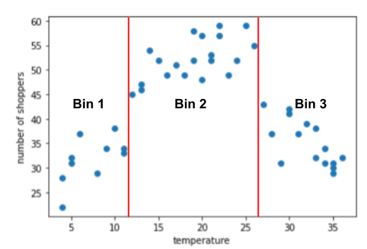
The graph suggests three clusters in the following subranges:
- Bin 1 is the temperature range 4-11.
- Bin 2 is the temperature range 12-26.
- Bin 3 is the temperature range 27-36.
The model learns separate weights for each bin.
Quantile bucketing
Quantile bucketing creates bucketing boundaries such that the number of examples in each bucket is exactly or nearly equal.
Scrubbing
Many examples in datasets are unreliable. You can write a program or script to detect any of the following problems:
- Omitted values
- Duplicate examples
- Out-of-range feature values
This is Scrubbing.
Qualities of good numerical features
- Clearly named: Not recommended:
house_age: 851472000; Recommended:house_age_years: 27 - Checked or tested before training: Bad
user_age_in_years: 224; OKuser_age_in_years: 24 - Sensible: A “magic value” is a purposeful discontinuity in an otherwise continuous feature.
Polynomial transforms
A Polynomial Transform is a technique used to map your original input features into a higher-dimensional space by generating polynomial combinations of the original features.
Steps of handling numerical Data
Visualize your data
Visualizations help you continually check your assumptions. Use Pandas for visualization:
- Working with Missing Data: pandas Documentation
- Visualizations pandas Documentation
Statistically evaluate your data
Use Pandas describe()
Find outliers
There are some common rule to find outliers. For example: When the delta between the 0th and 25th percentiles differs significantly from the delta between the 75th and 100th percentiles, the dataset probably contains outliers.
- The outlier can be due to a mistake.
- The outlier is a legitimate data point, you can keep these outliers in your training set. But extreme outliers can still hurt your model. You can delete the outliers or apply more invasive feature engineering techniques, such as clipping.
Numerical data Best practices
Best practices for working with numerical data:
- Remember that your ML model interacts with the data in the feature vector, not the data in the dataset.
- Normalize most numerical features.
- If your first normalization strategy doesn’t succeed, consider a different way to normalize your data.
- Binning, also referred to as bucketing, is sometimes better than normalizing.
- Considering what your data should look like, write verification tests to validate those expectations. For example:
- The absolute value of latitude should never exceed 90. You can write a test to check if a latitude value greater than 90 appears in your data.
- If your data is restricted to the state of Florida, you can write tests to check that the latitudes fall between 24 through 31, inclusive.
- Visualize your data with scatter plots and histograms. Look for anomalies.
- Gather statistics not only on the entire dataset but also on smaller subsets of the dataset. That’s because aggregate statistics sometimes obscure problems in smaller sections of a dataset.
- Document all your data transformations.
Categorical Data
Categorical Data is the Data which behave like categories. The numerical data can be Categorical Data. Because models can only train on floating-point values, Categorical Data need to be Encoded.
- How to encode categorical data?
- For low-dimensional categorical, one important concept is one-hot encoding.
- But for most of categorical data will be high-dimensional. Embedding is the big part of the encoding methods.
- Numerical data is often recorded by scientific instruments or automated measurements. Categorical data, on the other hand, is often categorized by human beings(gold labels) or by machine learning models(silver labels). Who decides on categories and labels, and how they make those decisions, affects the reliability and usefulness of that data.
Low-dimensional categorical features
Vocabulary encoding is for a low number of possible categories.
With a vocabulary encoding, the model treats each possible categorical value as a separate feature. During training, the model learns different weights for each category.
Index numbers
First you must convert each category string to a unique index number.
One-hot encoding
The next step in building a vocabulary is to convert each index number to its one-hot encoding.
In a one-hot encoding:
- Each category is represented by a vector (array) of
Nelements, whereNis the number of categories. For example, if car_color has eight possible categories, then the one-hot vector representing will have eight elements. - Exactly one of the elements in a one-hot vector has the value 1.0; all the remaining elements have the value 0.0.
It is the one-hot vector, not the string or the index number, that gets passed to the feature vector. The model learns a separate weight for each element of the feature vector.
sparse representation
Sparse representation means storing the position of the 1.0 in a sparse vector. For example, the one-hot vector for “Blue” is: [0, 0, 1, 0, 0, 0, 0, 0] Since the 1 is in position 2 (when starting the count at 0), the sparse representation for the preceding one-hot vector is: 2
Sparse representation consumes far less memory than the eight-element one-hot vector.
Importantly, the model must train on the one-hot vector, not the sparse representation.
High-dimensional categorical features
Some categorical features have a high number of dimensions, like words_in_english.
When the number of categories is high, one-hot encoding is usually a bad choice.
- Embeddings are usually a much better choice. Embeddings substantially reduce the number of dimensions, which benefits models in two important ways:
- The model typically trains faster.
- The built model typically infers predictions more quickly. That is, the model has lower latency.
- Hashing (also called the hashing trick) is a less common way to reduce the number of dimensions.
What is feature crosses
Feature crosses are created by crossing two or more categorical or bucketed features of the dataset.
For example, consider a leaf dataset with the categorical features:
-
edges, containing valuessmooth,toothed, andlobed -
arrangement, containing valuesoppositeandalternate
The feature cross of these two features would be: {Smooth_Opposite, Smooth_Alternate, Toothed_Opposite, Toothed_Alternate, Lobed_Opposite, Lobed_Alternate}
feature crosses vs. polynomial transforms
Feature crosses are somewhat analogous to Polynomial transforms. Both combine multiple features into a new synthetic feature that the model can train on to learn nonlinearities.
- Polynomial transforms typically combine numerical data, while feature crosses combine categorical data.
- Like polynomial transforms, feature crosses allow linear models to handle nonlinearities. Feature crosses also encode interactions between features.
When to use feature crosses
- Domain knowledge can suggest a useful combination of features to cross. Without that domain knowledge, it can be difficult to determine effective feature crosses or polynomial transforms by hand.
- It’s often possible, if computationally expensive, to use neural networks to automatically find and apply useful feature combinations during training.